Kinematics: Displacement, Velocity, and Acceleration

Introduction

...there are subtleties—several of them. In the first place, what do we mean by time and space? It turns out that these deep philosophical questions have to be analyzed very carefully in physics, and this is not so easy to do. The theory of relativity shows that our ideas of space and time are not as simple as one might think at first sight. However, for our present purposes, for the accuracy that we need at first, we need not be very careful about defining things precisely. Perhaps you say, "That's a terrible thing—I learned that in science we have to define everything precisely." We cannot define anything precisely.

- Richard Feynman, Lectures on Physics

We start our study of physics with Newtonian mechanics: an investigation into the nature of motion. What do we mean by distance? speed? velocity? acceleration? How are these quantities related to space and time, position and movement? To answer these questions, we need to develop a way of analyzing motion. Our goals in the first two chapters of the text are to show how position in space over time can be mapped using coordinate systems and vectors. To simplify things, we start with motion where acceleration is constant (not changing) and the object is moving through space without rotating (changing position, but not orientation), a type of motion called translation.

The problems of distance and time

The fundamental questions of the natural universe occupied the Greeks of ancient Ionia and set the pattern for Western science. What is matter? What is motion? What is time? Ever since they posed these questions, we have been trying to understand and describe what happens when an object changes position. We all have a day-to-day understanding of motion, but when we start to look more closely at what it happening, we find that it is like playing with a Chinese finger puzzle: the more you tug, the tighter the concepts become.

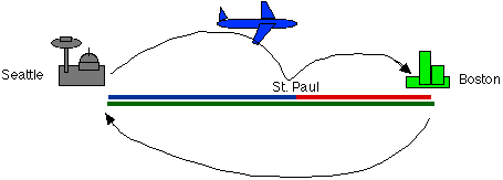
Let's take a simple, straightforward example of motion: several years ago, I had the opportunity to travel to Boston from Seattle on business. Disregarding all aspects of the matter involved (including the mass), let's consider what we can find out about the movement of one online teacher from one side of the country to the other and back again.

According to my ticket, I flew from Seattle to St. Paul, MN, a distance of about 1700 miles (blue line) in 223 minutes. I then changed planes, and flew to Boston, a distance of 1000 miles (red line), in 140 minutes. On the return trip, I flew (non-stop) a distance of 2700 miles (green line) in 250 minutes.

Scalar Quantities: Distance and speed

We use two concepts to talk about the separation of place in space. Distance is an amount of linear space that we cover when we travel from point A to point B. The total distance that I travelled on my trip was about 5400 miles. Displacement is distance from some particular location, or position relative to an origin and coordinate system. At the beginning of my trip, my displacement from Seattle was 0. While I was in Boston, my displacement was about 2700 miles. At the end of my trip, I was back where I started: my displacement from Seattle was 0.

The relationship when distance is divided by time is speed.

s = \frac{d}{t}

We measure it here in miles per minute, but most of our physics work will use international units of meters or kilometers and seconds. The important thing to note is that the units of speed are always units of distance divided by units of time. Normally we don't talk about units of time/units of distance; while you may want to do this in trip planning, physics has no special name for this relationship.

Vector Quantities: Displacement and velocity

Speed has a very close conceptual relative in velocity, which is displacement/time. Displacement has direction (which way?) as well as magnitude (how far?). Notice that we displacement will differ if I measure it from different origins or starting points. While I was traveling to Boston, my displacement from Seattle increased BUT my displacement from Boston decreased. D_SB = -D_BS, where S indicates Seattle and B Boston, and the order shows the direction I was flying. We have to take direction into account when we think about displacement.

Quantities with both magnitude and direction are called vectors and are used throughout physics to represent concepts such as displacement, velocity, acceleration, and various forces. Because the have direction, we generally use arrows above the letter variable for the vector, or print the vector in bold, to differentiate it from its scalar (magnitude only) quantity.

Scalar	Vector
x = distance	d= displacement
v = speed	v = velocity

Sometimes we map displacements using a Cartesian co-ordinate system, which may be familiar to you from algebra class. In this system, we can show displacement as a line along the x-axis:

This graph shows a displacement from 0 to 9. Such a displacement, often labeled Δ_x) is represented by an arrow: displacement is a vector. In general, when we have real situations, we move the coordinate system around so that we can use it conveniently. For motion in one dimension, we will always align our coordinates so that the motion parallels the X axis. Next week we will talk about representing motion in two dimensions.

Average and Instantaneous Quantities

So far, we have only considered the average speed or velocity of my plane, but obviously, the plane was not flying at 600+ miles per hour the entire trip. If it had, our entrance to the St. Paul/Minneapolis Airport would have made international news, Boeing and the NTSB would be investigating the result, and you would have someone else teaching this class. At some point over North Dakota or Minnesota, the plane began to slow down in order to make a safe landing.

Changes in velocity are called acceleration, and can occur in several ways.

We can speed the plane up, as on take-off. This positive acceleration increases the velocity.
We can slow the plan down, as when landing. This negative acceleration (sometimes called deceleration) decreases the velocity.
We can change the direction of the plane without changing its speed, as when going around very big, dark, menacing clouds full of lightning above Bismarck. This is still acceleration, since there is a change in velocity--it has a new direction.
We can have constantly changing acceleration of direction without change in speed, as when circling Logan Airport waiting for the storm to pass over and the tower to give us permission to land. We will talk about circular motion at length in a later chapter.
Note that in all the above cases, acceleration can be constant or it can vary.

Instantaneous Velocity

So far, we have been discussing average velocities and average accelerations, that is, changes that occur over some finite period of time. Sometimes it is important to know what the velocity is at a given instant of time. We represent instantaneous quantities by considering what happens to the quantity when the Δ_t factor goes to zero:

\lim_{Δ t \to 0} = \frac{Δ x}{Δ t} = v

Note that we can't simply set Δ_t to zero, because then Δ_x/Δ_t would blow up to infinity, which tells us nothing. We have to consider the entire function for Δ_x/Δ_t, using that special mathematics of functions limits called calculus.

Consider for a moment a velocity that is unchanging. We can represent the displacement at any moment as a straight line of the form (in our text's notation): x = vt + x₀ Those of you who have Cartesian coordinates firmly in mind may recognize this as exactly the same form as the standard linear equation: y = mx + b where +y is the distance up (vertically) from the origin and +x is the distance to the right, while m is the slope and b is the offset. If we put b=0, our line becomes y = mx and passes through the origin. The graph below shows three lines, each with b=0 and slopes of m = .1 (red), m = .3 (blue) and m = .5 (green). The bigger m is, the steeper the slope.

What happens to the line when m is 0? It becomes horizontal!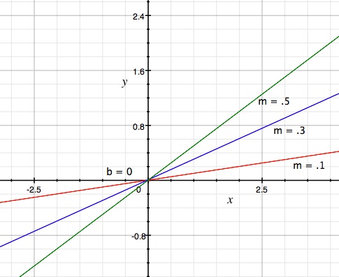

Now let's translate that back into our equation for displacement. Just to keep you from confusing x = the text's symbol for displacement with x = the distance along the horizontal coordinate in our graph, let's use d = distance.

Our distance equation is then d = vt + d₀.
We measure d up and down (along the y axis), with each tick = .2 units of distance. If it helps, think meters.
We measure t to the right (along the x axis), with each tick = .5 units of time. If it helps, think seconds.
Remember that slope = Δy/Δx, or in this case, Δd/Δt. But we've defined Δd/Δt as velocity, so the slope of our plotted line is the velocity!
The red line crosses the vertical line at .1 up (halfway to the .2 meters mark) at t = 1 seconds (two marks along the x axis). This means we've traveled .1 meters in 1 second -- and our speed is .1 meters/second.
The blue line crosses the vertical line at .3 up (halfway between the first and second .2 meters marks) at t = 1 seconds. This means we've traveled .3 meters in 1 second -- and our speed is .3 meters/second.
The green line crosses the vertical line at .5 up (halfway between the second and third .2 meters marks) at t = 1 seconds. This means we've traveled .5 meters in 1 second -- and our speed is .5 meters/second.

We could change the origin, and then we'd have the situation where d = vt + d₀:

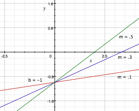We've looked at the situation where d₀ = 0 — we start at the origin. We can also start with an initial displacement. If we start at d₀ = -1 (below the horizontal line), then we have to travel longer to get to the same spot. Note that the m=.3 line reaches .1 at 4 seconds now, instead of just over 3 seconds as it did before, so where we start measuring distance from matters.

So far, we have a constant velocity in all three cases — so the slope doesn't change. The instantaneous velocity and the average velocity are the same. Now let's look briefly at what happens when velocity is changing because it is under acceleration. We'll spend a lot more time on the physics of this in the next web lecture; for now, we just want to look at the math so that we can understand the different between instantaneous and average speeds.

Here's a graph of a projectile's path up, and then down, under the force of gravity. Because gravity is decelerating the object while it is rising, and accelerating it while it is falling, the path of the object (black) where distance is plotted along the y-axis and time along the x-axis, is a curve. The slope of the curve is constantly changing. We've plotted a line tangent to the slope at one point in time, about x = 0.45. The slope of the tangent line is the instantaneous velocity. If we move along the path plot even a little, the tangent to our new point would change.

If you move up the line, how does the slope change? If you move down the line, how does the slope change? What does that tell you about how the velocity of the projectile is changing?

Summing up

Let's document the quantities we have discussed so far.

Position at time 0	$x_{0}$
Position at time t	$x_{1}$
Distance	${\| x}_{1} - x_{0} \|$ (absolute value; we don't care about direction in distance)
Displacement	$x_{1} - x_{0}$
Average velocity	$\frac{x_{1} - x_{0}}{t_{1} - t_{0}} = \frac{Δ x}{Δ t} = v$
Velocity at time 0	$v_{0}$
Velocity at time t	$v_{1}$
Speed	$\frac{\| x_{1} - x_{0} \|}{t_{1} - t_{0}}$
Average acceleration	$\frac{v_{1} - v_{0}}{t_{1} - t_{0}} = \frac{Δ v}{Δ t} = a$

Using these quantities and relationships, we can derive a number of new relationships; I'm not going to do that here, because it is covered in your text. Be sure that you understand how the derivations work.

Practice with the Concepts

Use Physics Classroom Distance and Displacement Lesson to help you understand how the two are related but different concepts.
Take a look at these oPhysics Velocity vs. Time graphs. Note how velocity changes when acceleration is 0, less than 1, and greater than one. What is the direction of the slope? How is the area under the slope related to the distance traveled during the period of constant acceleration?
Now use the oPhysicsPosition, Velocity, and Acceleration vs. Time Graphs. Change the velocity points to see how position and acceleration change.
Use the Acceleration in One Dimension graph to explore how changes to initial values for position, velocity, or acceleration change the other two related values.
Consider the flight of a baseball ricocheting from the bat of a home run slugger. The ball leaves the pitcher's hand, strikes the bat, soars out over center field, and drops into the upper deck. Where is the vertical velocity of the ball zero? Where is the horizontal velocity of the ball zero? (Click on the button to check your reasoning once you have worked out your answer.)

Discussion Points

What is the difference between vector and scalar quantities [for example, between distance and displacement]?
What is the difference between average and instantaneous measurements or quantities?
What do we mean by "limiting situations"? How can the limit case of a given event be used to explore what is going on?

© 2005 - 2025 This course is offered through Scholars Online, a non-profit organization supporting classical Christian education through online courses. Permission to copy course content (lessons and labs) for personal study is granted to students currently or formerly enrolled in the course through Scholars Online. Reproduction for any other purpose, without the express written consent of the author, is prohibited.

Physics

Chapter 2: 1-5 Displacement and Velocity